Standard Gaussian Processes • GPCERF

library(GPCERF)
library(ggplot2)

In this vignette, we present an example of using standard Gaussian processes approach in GPCERF to estimate the exposure response function (ERF) of a continuous exposure based on simulated data. We use a synthetic data generation function from the R package CausalGPS.

Generate Synthetic Data

We first generate a synthetic dataset with six covariates, one continuous exposure and one outcome. We consider two types of conditional distributions (normal and student’s t) of the exposure given covariates. For more details of the synthetic data generation, see this document. We then use a function tru_R to derive the actual ERF of this population at w=seq(0,20,0.1).

set.seed(134)
# Generate dataset with a normally distributed exposure given covariates
data_sim_normal <- generate_synthetic_data(sample_size = 400,
                                           outcome_sd = 10,
                                           gps_spec = 1)

# Generate dataset with a t-distributed with 2df exposure given covariates
data_sim_t <- generate_synthetic_data(sample_size = 400,
                                      outcome_sd = 10,
                                      gps_spec = 2)

tru_R <- function(w, sim_data) {
  design_mt <- model.matrix(~cf1 + cf2 + cf3 + cf4 + cf5 + cf6 - 1,
                            data = sim_data)
  mean(apply(design_mt, 1, function(x) {
    -10 - sum(c(2, 2, 3, -1, 2, 2) * x) -
      w * (0.1 - 0.1 * x[1] + 0.1 * x[4] + 0.1 * x[5] + 0.1 * x[3] ^ 2) +
      0.13 ^ 2 * w ^ 3
  }))
}

plot_fun <- function(object, ...) {
    # extract data
  tmp_data <- data.frame(w_vals = object$posterior$w,
                         mean_vals = object$posterior$mean,
                         sd_vals = object$posterior$sd)

  g1 <- ggplot2::ggplot(tmp_data) +
       ggplot2::geom_ribbon(ggplot2::aes(.data$w_vals,
                                y = .data$mean_vals,
                                ymin = .data$mean_vals - 1.96 * .data$sd_vals,
                                ymax = .data$mean_vals + 1.96 * .data$sd_vals),
                                fill = "blue", alpha = 0.25) +
        ggplot2::geom_line(ggplot2::aes(.data$w_vals, .data$mean_vals),
                           color = "blue", size = 1) +
        ggplot2::theme_bw() +
        ggplot2::ggtitle("Estimated CERF (gp) with credible band (1.96sd)") +
        ggplot2::xlab("Exposure level") +
        ggplot2::ylab("Population average counterfactual outcome")

  return(g1)
}

erf_tru_normal <- sapply(seq(0, 20, 0.1), function(w) tru_R(w, data_sim_normal))
erf_tru_t <- sapply(seq(0, 20, 0.1), function(w) tru_R(w, data_sim_t))

Estimate ERF with standard Gaussian Processes

Train GPS Model

GPCERF will first convert the covariate values into a single composite score (GPS) and then use it to fit the Gaussian processes. We use the GPS estimation function in CausalGPS (see here) to get the GPS model that maps covariates into GPS.

gps_m_normal <- estimate_gps(cov_mt = data_sim_normal[, -(1:2)],
                             w_all = data_sim_normal$treat,
                             sl_lib = c("SL.xgboost"),
                             dnorm_log = FALSE)
#> Loading required package: nnls

gps_m_t <- estimate_gps(cov_mt = data_sim_t[, -(1:2)],
                        w_all = data_sim_t$treat,
                        sl_lib = c("SL.xgboost"),
                        dnorm_log = FALSE)

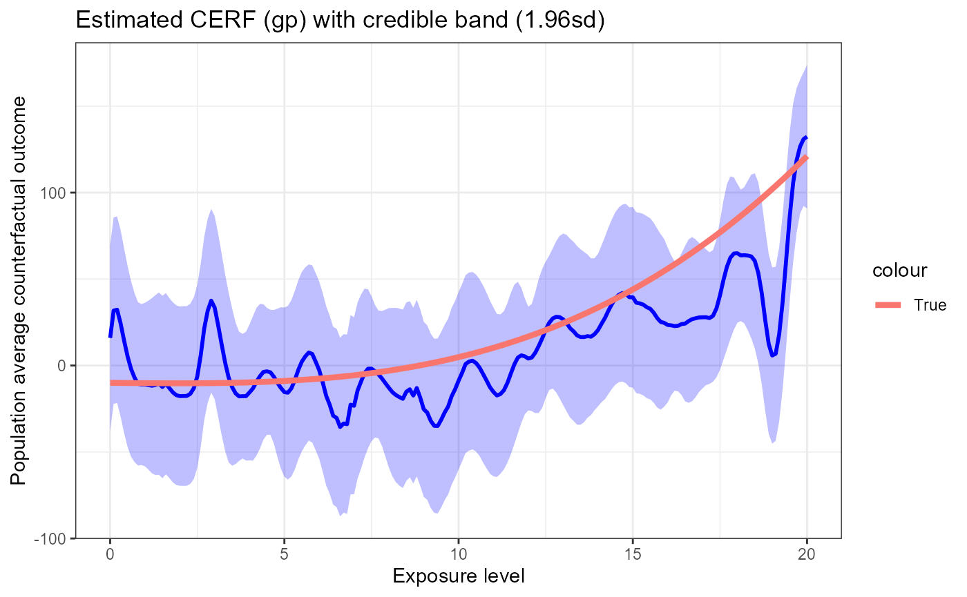
We then use estimate_cerf_gp to estimate the ERF of the exposure w. We estimate the ERF at w = seq(0,20,0.1). The estimated ERF as well as its pointwise 95% credible band is visualized with a call to plot. We also plot the actual ERF on top of the estimated ERF.

Normally Distributed Exposure

w_all <- seq(0, 20, 0.1)

gp_res_normal <- estimate_cerf_gp(data_sim_normal,
                                  w_all,
                                  gps_m_normal,
                                  params = list(alpha = c(0.1),
                                                beta = 0.2,
                                                g_sigma = 1,
                                                tune_app = "all"),
                                  outcome_col = "Y",
                                  treatment_col = "treat",
                                  covariates_col = paste0("cf", seq(1,6)),
                                  nthread = 1)
plot_fun(gp_res_normal) +
  geom_line(data = data.frame(w = w_all, y = erf_tru_normal),
            aes(x = w, y = y, color = "True"), size = 1.5)
#> Warning: Using `size` aesthetic for lines was deprecated in ggplot2 3.4.0.
#> ℹ Please use `linewidth` instead.
#> This warning is displayed once every 8 hours.
#> Call `lifecycle::last_lifecycle_warnings()` to see where this warning was
#> generated.

We can see that the estimated curve follows the true ERF closely and the 95% credible band completely covers the true ERF.

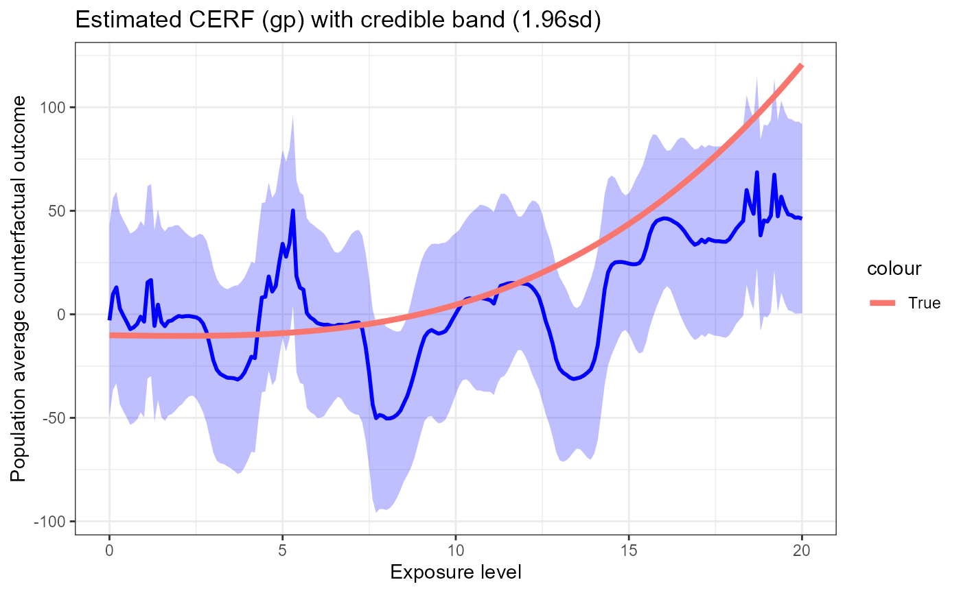
T-distributed Exposure

gp_res_t <- estimate_cerf_gp(data_sim_t,
                             w_all,
                             gps_m_t,
                             params = list(alpha = c(0.1),
                                           beta = 0.2,
                                           g_sigma = 1,
                                           tune_app = "all"),
                             outcome_col = "Y",
                             treatment_col = "treat",
                             covariates_col = paste0("cf", seq(1,6)),
                             nthread = 1)
plot_fun(gp_res_t) +
  geom_line(data = data.frame(w = w_all, y = erf_tru_t),
            aes(x = w, y = y, color = "True"), size = 1.5)

The results look very similar to the case where the exposure is normally distributed. The only difference might be that when the exposure is t-distributed, the estimated curve tends to be less smooth.