CausalGPS | Example 1
Contents
CausalGPS | Example 1
Matching with parametric GPS model
In this example, we will use the CausalGPS R package to generate pseudo population based on parametric GPS model. We use synthetic Medicare data that is available in the package. All processing are done in R.
Step 1: Install and load the package
install.packages("CausalGPS")
library(CausalGPS)
Step 2: Load the data
data("synthetic_us_2010", package = "CausalGPS")
synthetic_us_2010$cdc_mean_bmi[synthetic_us_2010$cdc_mean_bmi > 9000] <- NA
data <- synthetic_us_2010

confounders_s1 <- c("cs_poverty","cs_hispanic",
                    "cs_black",
                    "cs_ed_below_highschool",
                    "cs_median_house_value",
                    "cs_population_density",
                    "cdc_mean_bmi","cdc_pct_nvsmoker",
                    "gmet_mean_summer_tmmx",
                    "gmet_mean_summer_rmx",
                    "gmet_mean_summer_sph",
                    "cms_female_pct", "region"
)

data$region <- as.factor(data$region)
Step 3: Generate Pseudo Population
set.seed(574)
ps_pop_obj_1 <- generate_pseudo_pop(data$cms_mortality_pct,
                                    data$qd_mean_pm25,
                                    data.frame(data[, confounders_s1, drop=FALSE]),
                                    ci_appr = "matching",
                                    gps_model = "parametric",
                                    bin_seq = NULL,
                                    trim_quantiles = c(0.25 ,
                                                       0.99),
                                    optimized_compile = TRUE,
                                    use_cov_transform = TRUE,
                                    sl_lib = c("m_xgboost"),
                                    params = list(xgb_nrounds=seq(10,60),
                                                  xgb_eta=seq(0.04, 0.4, 0.02)),
                                    nthread = 12,
                                    covar_bl_method = "absolute",
                                    covar_bl_trs = 0.1,
                                    covar_bl_trs_type= "maximal",
                                    max_attempt = 10,
                                    matching_fun = "matching_l1",
                                    delta_n = 0.1,
                                    scale = 1)
In the previous code, we trimmed data using trim_quantiles. This helps to focus on common support range. m_ in m_xgboost stands for modified xgboost library. So we can pass a range of hyperparameter with xgb_ prefix. Covariate balance has 3 options including method (which only absolute has been implemented so far), threshold (covar_bl_trs) and threshold type (covar_bl_trs_type) which includes mean, median, and maximal. max_attempt is the maximum number of attempts to generate pseudo population. matching_fun is the matching function (only matching_l1 has been implemented so far). delta_n is the size of caliper and scale is a specified scale parameter to control the relative weight that
is attributed to the distance measures of the exposure versus the GPS.
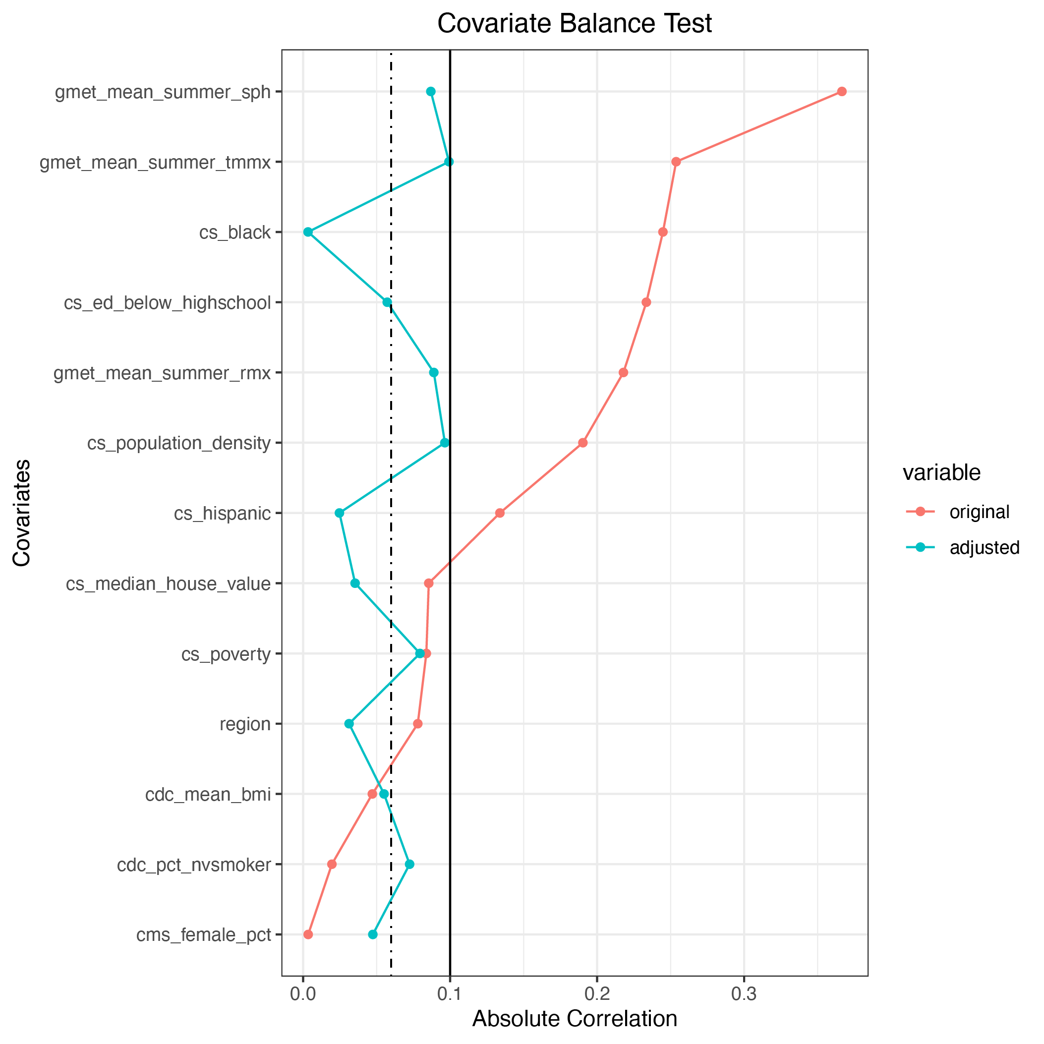
After 6 iterations, a covariate balance is achieved one can run summary to see the summary of the results.
summary(ps_pop_obj_1)
--- CausalGPS pseudo population object summary ---
Pseudo population met the covariate balance requirement:  TRUE
Absolute correlation of the original data:
   mean:     0.151
   median:   0.134
   maximal:  0.367

 cs_poverty : 0.084
 cs_hispanic : 0.134
 cs_black : 0.245
 cs_ed_below_highschool : 0.234
 cs_median_house_value : 0.085
 cs_population_density : 0.190
 cdc_mean_bmi : 0.047
 cdc_pct_nvsmoker : 0.020
 gmet_mean_summer_tmmx : 0.254
 gmet_mean_summer_rmx : 0.218
 gmet_mean_summer_sph : 0.367
 cms_female_pct : 0.003
 region : 0.078

 Absolute correlation of the pseudo population:
   mean:     0.060
   median:   0.057
   maximal:  0.099

 cs_poverty : 0.079
 cs_hispanic : 0.025
 cs_median_house_value : 0.003
 cdc_mean_bmi : 0.057
 cdc_pct_nvsmoker : 0.035
 gmet_mean_summer_tmmx : 0.096
 gmet_mean_summer_sph : 0.055
 cms_female_pct : 0.072
 cs_black : 0.099
 cs_ed_below_highschool : 0.089
 cs_population_density : 0.087
 gmet_mean_summer_rmx : 0.047
 region : 0.031

 Hyperparameters used for the select population:
 xgb_nrounds : 21
 xgb_max_depth : 6
 xgb_eta : 0.32
 xgb_min_child_weight : 1
 xgb_verbose : 0

Number of data samples:  2299
Number of iterations:  6
--- *** ---
It is important to note that the package ignores any data with missing values. As a result, number of data samples are different from the original data. We can also plot the covariate balance.
Now, we can conduct the analysis using the pseudo population.
set.seed(168)
erf <- estimate_npmetric_erf(m_Y = ps_pop_obj_1$pseudo_pop$Y,
                             m_w = ps_pop_obj_1$pseudo_pop$w,
                             counter_weight = ps_pop_obj_1$pseudo_pop$counter_weight,
                             bw_seq = seq(0.2,10,0.05),
                             w_vals = seq(7,13, 0.05),
                             nthread = 12)